Mutual Information Neural Estimators

Mutual Information

As part of my work on Concept Bottleneck Models, I looked at mutual information and its estimation quite often!

Mutual Information is a metric for measuring the mutual dependence between two random variables. Specifically it tell us the information content gained about one random variable by observing the other. Given a pair of random variables $(X,Y)$ with joint distribution $P_{(X,Y)}$ and marginals $P_X$ and $P_Y$, we define the mutual information as the following:

$$ \begin{align} I(X;Y) &= D_{KL}(P_{(X,Y)} || P_X \otimes P_Y) \\ &= \int log \big( \frac{dP_{(X,Y)}}{d(P_X \otimes P_Y)}(x,y)\big) dP_{(X,Y)}(x,y) \end{align} $$

$D_{KL}$ is the Kullback–Leibler divergence. We can make use of the Radon-Nikodym derivative when the joint measure is continuous with respect to the product measure ($P_X \otimes P_Y$) to get the following expectation:

$$ \begin{align} I(X;Y) = \mathbf{E}_{P_{(X,Y)}}\bigg[\log\bigg(\frac{p(x,y)}{p(x)p(y)}\bigg)\bigg] \end{align} $$

This definition of mutual information is well-defined if and only if $P_{(X,Y)}$ is absolutely continuous with respect to the product measure. $D_{KL}$ is the Kullback-Leibler divergence and so the mutual information is just the KL divergence between the joint distribution of two random variables and the product of their marginals! Mutual information is both symmetric and non-negative (due to KL diverence).

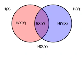
$$ \begin{align} I(X;Y) &= \mathbf{E}_{P_{(X,Y)}}\bigg[\log\bigg(\frac{p(x,y)}{p(x)p(y)}\bigg)\bigg] \\ &= \mathbf{E}_{P_{(Y, X)}}\bigg[\log\bigg(\frac{p(y,x)}{p(y)p(x)}\bigg)\bigg] = I(Y;X) \end{align} $$

We can also define mutual information in terms of entropies. The entropy $H(.)$ of a random variable is a measure of the level of uncertainty associated with the variable averaged over all possible outcomes, the discrete and continuous versions are provided below:

$$ \begin{align} H(X) &= - \sum_{x} p(x) \log p(x) \\ h(X) &= - \int_{-\infty}^{\infty} f(x) \log f(x) \, dx \end{align} $$

We can use the above to define mutual information as follows:

$$ \begin{align} I(X;Y) = H(X) - H(X|Y) \end{align} $$

The expression above has strong links to deep learning, if we think about the cross-entropy loss function being applied during training, the backpropagation algorithm acts on the hidden layers to actively maximize the Mutual Information between those hidden layers ($Z$) and the target labels ($Y$). This also motivates the use of information bottleneck method to optimally compress our input data to retain only the features most relevant for predicting the output.

There are lots of older knn based MI estimation algorithms, however here I only focus on neural network based approaches which can be useful given they are end-to-end differentiable, therefore allowing for direct minimisation/maximisation during training.

MINE

Mutual Information Neural Estimators (MINE) were first introduced in 2018 as a estimator of the mutual information between random variables through gradient descent over a neural network.

MINE makes use of the Donsker-Varadhan representation of the KL divergence shown below:

Theorem (DV representation of the KL divergence): The Kullback Leibler divergence admits the dual representation shown below:

$$ D_{KL}(\mathbb{P} || \mathbb{Q}) = \sup\limits_{T : \Omega \to \mathbb{R}} \mathbb{E}_{\mathbb{P}}[T] - \log(\mathbb{E}_{\mathbb{Q}}[e^T]) $$

where the supremum is taken over all possible functions $T$ such that the two expectations are finite.

MINE uses of the DV representation above and instead of searching over all possible functions, restricts itself to a family of functions $\mathcal{F}$ which is parameterised by a neural network $T_\theta : \mathcal{X} \times \mathcal{Z} \xrightarrow[]{} \mathbb{R}$ with parameters $\theta \in \Theta$ and then make use of this statistics network to determine the neural information measure which is a lower bound for the true mutual information. $X$ and $Z$ are often random variables whose true distributions are not known and so $\mathbb{P}$ is approximated through the empirical distribution associated to $n$ i.i.d samples denoted $\hat{\mathbb{P}}^{(n)}$. MINE therefore provides the following lower bound estimation for the mutual information between two random variables $X$ and $Z$ as follows:

$$ \begin{align} \widehat{I_{\hat{\theta}}(X, Z)}_{n} &= \sup\limits_{\theta \in \Theta} \mathbb{E}_{\mathbb{P}^{(n)}_{XZ}}[T_\theta] - \log(\mathbb{E}_{\mathbb{P}^{(n)}_{X} \otimes \mathbb{P}^{(n)}_{Z}}[e^T_{\theta}]) \\ &\leq I(X; Z) \end{align} $$

Often when we don’t have the data generating process we can get samples from the marginal distributions by shuffling the order of one of the r.vs in the input. We do this so that our shuffled r.v is now independent of the other and so we can assume we have samples according to $P_XP_Y$

If we take gradients w.r.t our neural network parameters $\theta$ we end up with the following gradient:

$$ \hat{G}_B = \mathbf{E}_B[\nabla_{\theta}T_{\theta}] - \frac{\mathbf{E}_B[\nabla_{\theta}T_{\theta}e^{T_{\theta}}]}{\mathbf{E}_B[e^{T_{\theta}}]} $$

When we actually implement this don’t have access to the “full expectation” and have batch $B$ and so we get the following from gradient descent:

$$ \begin{align} &\nabla_{\theta}\bigg[\frac{1}{n}\sum_{i=1}^n T_{\theta} - \log(\frac{1}{n}\sum_{i=1}^ne^{T_{\theta}})\bigg] \\ & \frac{1}{n} \sum_{i=1}^n \nabla_{\theta}T_{\theta} - \frac{\sum_{i=1}^n \nabla_{\theta} T_{\theta} e^{T_{\theta}}}{\sum_{i=1}^n e^{T_{\theta}}} \end{align} $$

This is a biased gradient as $\mathbf{E}[\frac{A}{B}] \neq \frac{\mathbf{E}[A]}{\mathbf{E}[B]}$ if we use batch based optimisation techniques. Ratios of correlated random variables are often biased as we can see if we take a taylor expansion around their means:

$$ \mathbf{E}[\frac{A}{B}] \approx \frac{\mu_A}{\mu_B} - \frac{Cov(A,B)}{\mu_B^2} + \frac{\mu_A Var(B)}{\mu_B^3} $$

Clearly in our case term 2 is two correlated random variables which we have in our case.

We can fix this bias by using a exponential moving average (they do this in the paper). We introduce a variable $v$ which is updated throughout as folllows:

$$ v_{new} = (1 - \alpha)v_{old} + \alpha\bigg( \frac{1}{n} \sum_{i=1}^n e^{T_{\theta}(x_i, \bar{z}_i)} \bigg) $$

$\alpha$ is a learning rate for updates and we now use the following for our gradient estimate:

$$ \hat{G}_B = \frac{1}{n} \sum_{i=1}^n \nabla_{\theta}T_{\theta} - \frac{\sum_{i=1}^n \nabla_{\theta} T_{\theta} e^{T_{\theta}}}{v_{new}} $$

By introducing $v_{new}$, we now have a numerator calculated from current batch $B$ whereas the denominator is using historical samples (including current) which are all independently sampled, this decouples the numerator and the denominator. This covariance between the two massively decreases.

$$\begin{align} \text{Cov}\bigg(v_{new}, \sum_{i=1}^n \nabla_{\theta} T_{\theta} e^{T_{\theta}}\bigg) &= \text{Cov}\bigg((1 - \alpha)v_{old} \\ &\quad + \alpha\left( \frac{1}{n} \sum_{i=1}^n e^{T_{\theta}(x_i, \bar{z}_i)} \right), \sum_{i=1}^n \nabla_{\theta} T_{\theta} e^{T_{\theta}}\bigg) \nonumber \\ &= (1 - \alpha)\text{Cov}\left(v_{old}, \sum_{i=1}^n \nabla_{\theta} T_{\theta} e^{T_{\theta}}\right) \\ &\quad + \alpha \text{Cov}\left(\frac{1}{n} \sum_{i=1}^n e^{T_{\theta}(x_i, \bar{z}_i)}, \sum_{i=1}^n \nabla_{\theta} T_{\theta} e^{T_{\theta}}\right) \nonumber \end{align}$$

Since $v_{old}$ is calculated on previous independent samples (conditioned on $\theta$) from $\sum_{i=1}^n \nabla_{\theta} T_{\theta}e^{T_{\theta}}$ and so this covariance term vanishes to zero, the second term covariance causes the bias but now it is multiplied by $\alpha$ and so this bias massively decreases.

Our third term in the Taylor expansion ($Var(v_{new})$) can also be shown to be much smaller from some standard EMA results:

$$ Var(v_{new}) \approx \frac{\alpha}{2 - \alpha }Var(B_{exp}) $$

$B_{exp}$ is used just the current batch in the denominator like in the original expression. Now we have mostly corrected our bias we can use our estimator for both estimation and control!

Pseudocode

$$\begin{array}{l} \hline \textbf{Algorithm 1: } \text{MINE with Moving Average Bias Correction} \\ \hline \textbf{Input: } \text{Dataset } \mathcal{D} = \{(x_i, z_i)\}_{i=1}^n, \text{ learning rate } \eta, \text{ smoothing } \alpha \\ \textbf{Initialize: } \text{Parameters } \theta, \text{ moving average } v \leftarrow 1 \\ \textbf{while } \theta \text{ has not converged do} \\ \quad \text{1. Sample a batch } B = \{(x_i, z_i)\}_{i=1}^k \text{ from } \mathcal{D} \\ \quad \text{2. Generate marginal batch } \bar{B} = \{(x_i, z_{\pi(i)})\}_{i=1}^k \text{ (shuffling } z) \\ \quad \text{3. Calculate marginal expectation: } B_{exp} = \frac{1}{k} \sum_{i \in \bar{B}} e^{T_\theta(x_i, z_i)} \\ \quad \text{4. Update moving average: } v \leftarrow (1-\alpha)v + \alpha B_{exp} \\ \quad \text{5. Estimate Gradient: } \\ \quad \quad \hat{G}_B \leftarrow \nabla_\theta \left[ \frac{1}{k} \sum_{i \in B} T_\theta(x_i, z_i) \right] - \frac{\nabla_\theta \left[ \frac{1}{k} \sum_{i \in \bar{B}} T_\theta(x_i, z_i) e^{T_\theta(x_i, z_i)} \right]}{v} \\ \quad \text{6. Update parameters: } \theta \leftarrow \theta + \eta \hat{G}_B \\ \textbf{end while} \\ \hline \end{array}$$

Toy Dataset

To play around with this model, I generate a synthetic toy dataset which allows for generating random variables with known mutual information. I define a 2d Gaussian:

$$ \begin{pmatrix} X \\ Z \end{pmatrix} \sim \mathcal{N}(\mu, \Sigma) $$

where $\Sigma$ is defined as follows:

$$ \Sigma = \begin{pmatrix} I_d & \rho I_d \\ \rho I_d & I_d \end{pmatrix} $$

For $d=1$ we get the following:

$$ \Sigma = \begin{pmatrix} 1 & \rho\\ \rho & 1 \end{pmatrix} $$

We therefore have that $X \sim \mathcal{N}(0,1)$, $Z \sim \mathcal{N}(0,1)$ and $Cov(X, Z) = \rho$. We can also use a known result for jointly gaussian variables that gives us a known mutual information:

$$ I(X; Z) = \frac{1}{2} log\frac{|\Sigma_X| | \Sigma_Z|}{|\Sigma|} $$

For our structure this simplifies to

$$ I(X;Z) = -\frac{d}{2} \log(1- \rho^2) $$

Results

I train both the biased and EMA corrected MINE variants over the following configurations:

$$ \rho \in [0.85, 0.9, 0.95, 0.99] $$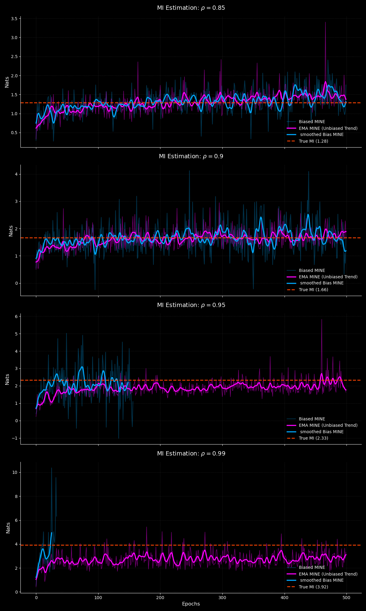

From our MI estimation plot we can see that as we increase $\rho$ the biased vanilla MINE very quickly diverges and produces inf estimates whilst our EMA MINE remains robust. The EMA based MINE also provides better estimates in expectation which is a direct result of the unbiased correction!

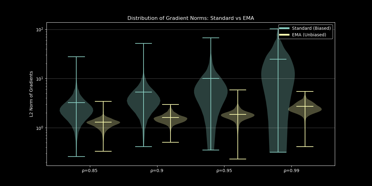
The uncorrected MINE very quickly diverges due to the massive gradient norms which increases with $\rho$ and this leads to the early divergence in MI estimates with norm of gradients reaching values of 100. This stems from the instability in the biased gradients second term!

All experiments ran are in the repo below: https://github.com/ahabisaax/MINE