Adaptive Random Walk Metropolis with Spectral Preconditioning

High-Level Overview
In Bayesian inference, we often need to sample from complex, high-dimensional posterior distributions that are non-conjugate. While MCMC algorithms like the Random Walk Metropolis (RWM) are the standard, they can fail when the posterior distribution has a difficult geometry—for example, if parameters are highly correlated.
This project implements a “smarter” RWM sampler that first learns the posterior’s geometry and then adapts its proposals, making it far more efficient at exploring these difficult, correlated spaces.
The Challenge: A Difficult, Misspecified Posterior
To test our sampler, we created a dataset with a known set of problems:
- Multicollinearity: The covariates in our design matrix $Z$ are deliberately correlated.
- Non-linear Data: One covariate, $x$, was sampled from a bimodal (U-shaped) distribution, creating sparse data in the middle.
- Skewed Errors: The noise was sampled from a Skew-Normal distribution, not a simple, symmetric Gaussian.
We then tried to fit two models to this data: a (wrong) misspecified linear model and the (correct) quadratic model that actually generated the data.
This setup creates a non-conjugate posterior distribution that is very difficult to sample from. The posterior for our true (quadratic) model is:
$$ p(\theta \mid y) \propto \left[ \prod_{i=1}^n \frac{2}{\sigma} \, \phi\left( \frac{y_i - (z_i^\top \beta + \gamma x_i^2)}{\sigma} \right) \, \Phi\left( \alpha \cdot \frac{y_i - (z_i^\top \beta + \gamma x_i^2)}{\sigma} \right) \right] \cdot \exp\left( -\frac{1}{2} \|\theta\|^2 \right) $$The Model: Adaptive RWM with Spectral Preconditioning
A standard Random Walk Metropolis (RWM) algorithm proposes new steps using a standard Gaussian:
$$ \theta^* = \theta^{(t)} + h \, \epsilon, \quad \epsilon \sim N(0, I) $$This is “isotropic”—it tries to move the same distance in all directions. This is inefficient for a posterior shaped like a long, narrow valley (which is what correlation creates).
Our model adds two enhancements:
Spectral Preconditioning: We first run a short “burn-in” chain to estimate the posterior covariance, $\widehat{\Sigma}$. We then use spectral decomposition ($\widehat{\Sigma} = Q\Lambda Q^T$) to find the posterior’s main axes of variance. We use this to “rotate and scale” our proposal to match the target’s geometry:
$$ \theta^* = \theta^{(t)} + h L_{spec}\epsilon \quad \text{(where } L_{spec} = Q\Lambda^{1/2} \text{)} $$Adaptive Step Size: We automatically tune the step size $h$ to target the optimal acceptance rate ($\alpha^* \approx 0.234$) using the Robbins-Monro algorithm. This ensures the chain is always exploring efficiently.
$$ h_{t+1} = h_t - \gamma_t(\hat{\alpha}_t - \alpha^*) $$
Our Approach & Results
We ran our adaptive, preconditioned RWM on both the misspecified linear model and the true quadratic model. We also ran a simple RWM and an adaptive-only RWM for comparison. We present traceplots of the quadratic and linear final models below:
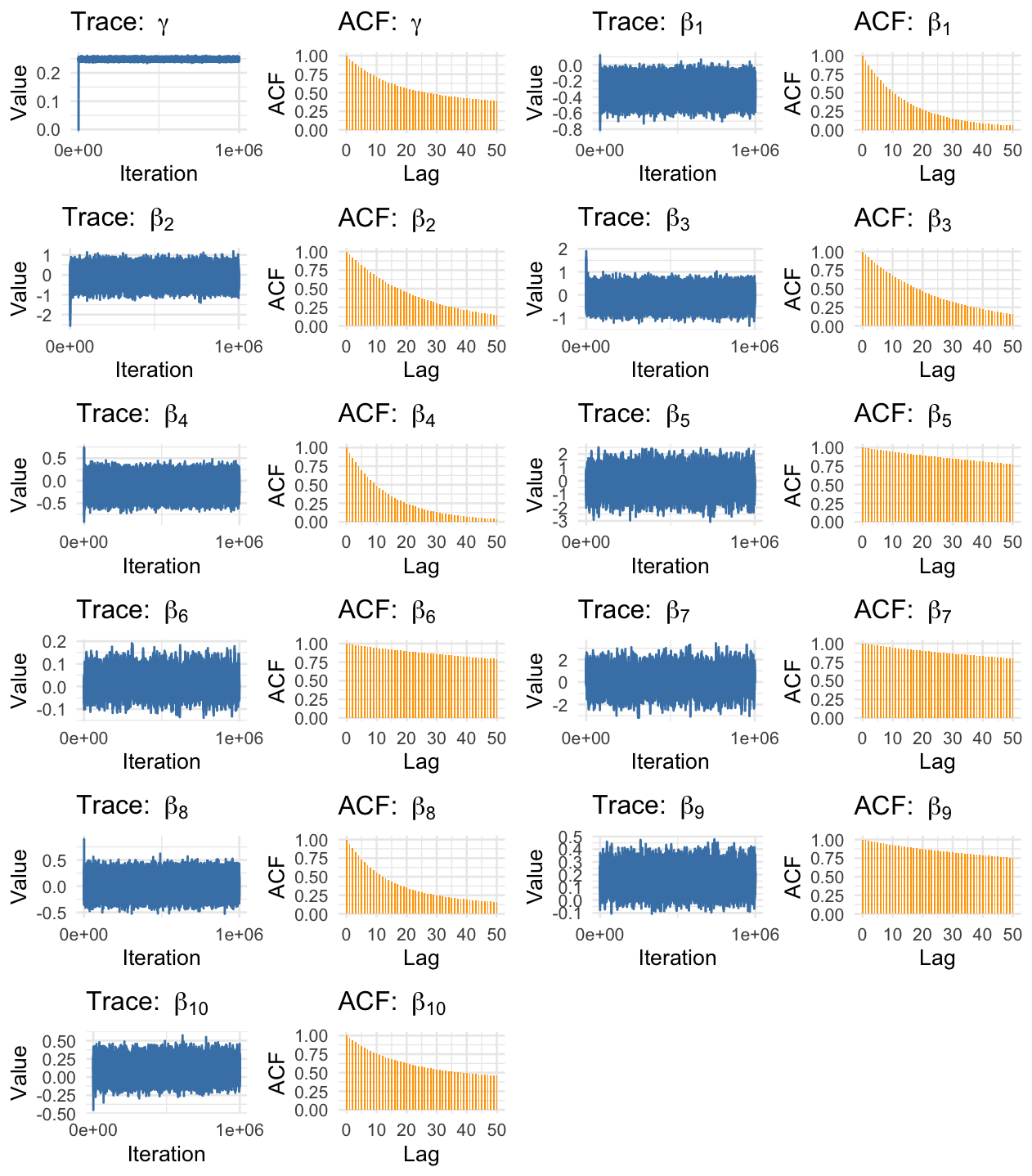
Traceplots for the quadratic model.
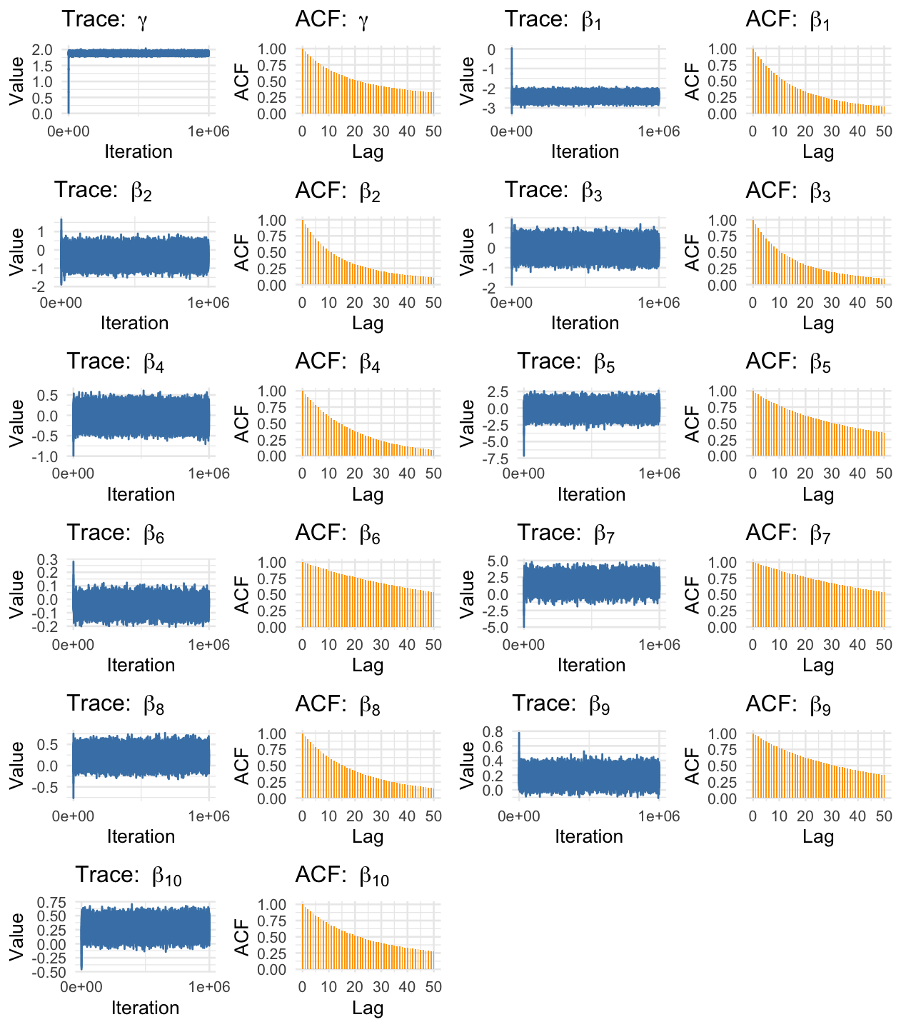
Traceplots for the linear model.
Preconditioning is the Key to Efficiency
The simple RWM and adaptive-only RWM completely failed, producing a minimum Effective Sample Size (ESS) of less than 10. They simply could not explore the correlated posterior.
Our preconditioned sampler achieved a minimum ESS of over 1900 for the most difficult parameters. Critically, the runtime was almost identical to the failed samplers. We achieved a >200x efficiency gain for free.
A Good Sampler Can’t Fix a Bad Model
The sampler’s efficiency also allowed us to see how bad the model misspecification was.
- The true quadratic model successfully recovered the true parameter for $\gamma$ (Estimate: 0.2484 vs. True: 0.25).
- The misspecified linear model was wrong. It compensated for the missing $x^2$ term by biasing $\gamma$ to 1.8797.
- Even using Bayesian Bagging on the linear model couldn’t fix it.